Approach Overview
The mask match algorithm is designed for picking multiple approximately flat objects simultaneously, using suction grippers with multiple suction groups.
Using a single suction group or picking a single object (with one or multiple suction groups) is also supported. For simplicity, this document always refers to multiple objects and multiple suction groups.
Simply put, the algorithm creates binary masks representing both the suction groups of the gripper and the objects for which a multi-object pick will be attempted. Then, by matching the masks of the gripper’s suction groups with the masks of the objects, it is possible to determine the position, rotation and suction group activation of the gripper, such that a stable pick is attempted, while maximizing the number of objects picked.
The details of the algorithm will be further explored in the subsequent sections.
The first step of the mask match algorithm is the creation of the masks representing the gripper. This step is done once in the lifetime of the command server, as it is constant between requests. This will be discussed in Representation of the GripperRepresentation of the Gripper.
With each request the algorithm expects a set of contact surfaces and associated object detections. These will be used to reason about how the gripper will engage with the scene.
It is expected that all of the gripper’s suction groups make contact with the objects on the same 'imaginary' planar surface (which can span multiple objects). As such, the extracted contact surfaces should be extracted from the objects in such a way that it is possible for the gripper to simultaneously make contact with all of them. Each set of contact surfaces will contain at most a single plane from each object.
Each plane in the contact surfaces' set gets its own unique binary mask representation, based on a configured pixel size. This will be discussed in Representation of the ObjectsRepresentation of the Objects.
Several pick proposals are computed, such that each of the objects associated with the contact surfaces' sets described above might be picked. This implies determining the position and rotation of the gripper, relative to the objects, in a way that it is possible to activate a combination of the gripper’s suction groups such that a stable pick of multiple objects is achieved. Multiple pick proposals are computed by contact surfaces' set, with each being scored based on multiple criteria. This will be discussed in Pick Proposals ComputationPick Proposals Computation.
The computed pick proposals are then returned to be handled by the pick planner.
The bulk of the mask match algorithm can run on either CPU or GPU. Running on GPU provides significantly faster execution. This behaviour can be controlled via the execution_device_index flag. Use execution_device_index < 0 for executing on the CPU and execution_device_index = <GPU device ID> for executing on the GPU device corresponding to the specified identifier. The id of a GPU device can be determined by running nvidia-smi on the command line.
Detailed Approach
Representation of the Gripper
The representation of a single gripper takes into consideration several aspects, such as the definition of the gripper itself, the desired gripper rotations and the size of the pixels used in the representation.
Simply put, each gripper will have one representation, encompassing all relevant gripper rotations and suction group combinations. For further details please read the collapsed section below.
| Gripper Definition |The definition of the gripper and its components is always done, either directly or indirectly, relative to the reference frame of an arbitrary grasp pose (indirect component definitions are done w.r.t. other components that are somehow defined relative to the grasp pose). For further clarification, please check the robot module.
| Gripper Rotations |Only gripper rotations about the z-axis of the default reference frame of the gripper are considered. The default reference frame of the gripper has the z-axis of its orientation pointing into the target objects. Its x-axis is aligned with the longest side of the tightest bounding box that can be fit around the combined planar surfaces under consideration for a pick.
TODO: Add visualization once standalone exists.
The mask match algorithm will consider number_linearly_spaced_rotations equally spaced rotations (in the range [0, 2*PI)) plus any rotation angles specified via specific_rotations.
| Pixel Size |The pixel size, configured via pixel_size, refers to the length, in SI units, of the side of an individual pixel used for the representations. Pixels are assumed to be square and all pixels have the same dimensions.
A lower pixel size will mean that the mask match algorithm will perform a more fine grained observation of where to place the gripper, potentially yielding better poses. However, this also implies that more computation will need to take place. Therefore, it is essential to find a pixel size that provides a good balance between accuracy and computation.
For creating the gripper representation for a given pixel size two main steps take place:
- Identification of the dimensions of the representation and creation of an empty canvas.
- Filling in the representation on the canvas.
Representation Dimensions
The dimensions of the representation need to be computed before the representation itself can be created. This is achieved by identifying the limits of the representation of each individual gripper component, given the pixel size and the condition that the reference frame of the gripper will be located at the very center of the representation. This is ensured by enforcing that the representation has odd sized sides (in terms of number of pixels). Additionally, for simplicity, the representation is made to be a square.
Given these conditions, the pose of each component is computed in the default reference frame of the gripper (i.e., the pose for which its x-axis is aligned with the long side of the object). The orientation of the default reference frame of the gripper is aligned with the representation’s x-axis and y-axis (default image coordinates). Note that a gripper rotation can already be considered during this step, which will influence the pose of the component relative to the default reference frame.
Having the default reference frame based pose of the component of the rotated gripper, the limits of the component are determined in terms of pixel coordinates, given the component’s geometric shape. For example, for a cylindrical geometric body, that will be its center ± its radius along each of the representation’s coordinate axes. This yields a bounding box for the component, relative to the centre of the gripper (i.e., the center of the representation).
Computing the full size of the representation consists of computing the union box of all its components, over all suction groups and gripper rotations (followed by ensuring it is an odd-sized square). In the end, a 0-filled-tensor is created, with the shape: [num_gripper_rotations, num_suction_groups, representation_size, representation_size]
Filling the Empty Representation
Filling the representation is done by a similar approach.
For each rotation and suction group combination, the pose of each suction group component is computed in the default reference frame. Then, each representation pixel is tested for whether its center (in non pixel coordinates) would be encompassed by the component’s geometric shape. If yes, then the pixel is set to 1, otherwise it will be left as 0.
In fact, only the representation’s pixels within the component’s bounding box are tested for, as all others would be left at 0 anyway.
Compressing the Representation
Since the set of representations of the gripper’s suction groups can be the same at different gripper rotations, there is no need to keep individual representations in those cases. This allows for compressing the overall gripper representation, such that some computational cost can be avoided when performing the tensorial reasoning part of the algorithm. The compression itself is best visualized via an example:
A gripper with 2 suction groups (A and B), each one a mirror of the other w.r.t. some axis, and 4 gripper rotations under consideration, 0°, 90°, 180° and 270°.
In this case, the representation of suction group A for 0° will be the same as the representation of suction group B for 180°, and vice-versa. The same happens between 90° and 270°.
This means that the set of suction group representations for 0° is the same as the set of suction group representations for 180° (remember that sets are unordered). The same happens between 90° and 270°.
Therefore, only two of the rotations' representations need to be kept, as long as the rotations and the ordered suction group indices they map to are tracked. In this case, if the representations of the rotation for 0° and 90° are kept, the following mapping would also need to be known:
representation-index-0:
    rotation-index-0 (can be remapped to   0° later): [A, B]
    rotation-index-2 (can be remapped to 180° later): [B, A]
representation-index-1:
    rotation-index-1 (can be remapped to  90° later): [A, B]
    rotation-index-3 (can be remapped to 270° later): [B, A]
Note that instead of A/B, the suction group indices would actually be kept, yielding something like:
representation-index-0:
    rotation-index-0 (can be remapped to   0° later): [0, 1]
    rotation-index-2 (can be remapped to 180° later): [1, 0]
representation-index-1:
    rotation-index-1 (can be remapped to  90° later): [0, 1]
    rotation-index-3 (can be remapped to 270° later): [1, 0]
Properties of Active Suction Groups
At later stages of the algorithm, Mask Match requires some information about how the active suction groups interact with one another. In order to do so, the representation for all elements of the power set of the possible combinations of active suction groups is computed, for all indices of the compressed representation, so that different properties can be computed based on them.
For example, given the following compressed representation of a mock gripper:
// COMPRESSED REPRESENTATION INDEX 0
//     SUCTION GROUP 0               SUCTION GROUP 1                 SUCTION GROUP 2
0.0, 0.0, 0.0, 1.0, 1.0,        1.0, 1.0, 0.0, 0.0, 0.0,        0.0, 0.0, 0.0, 0.0, 0.0,
0.0, 0.0, 0.0, 1.0, 1.0,        1.0, 1.0, 0.0, 0.0, 0.0,        0.0, 0.0, 0.0, 0.0, 0.0,
0.0, 0.0, 0.0, 0.0, 0.0,        0.0, 0.0, 0.0, 0.0, 0.0,        0.0, 0.0, 0.0, 0.0, 0.0,
0.0, 0.0, 0.0, 0.0, 0.0,        0.0, 0.0, 0.0, 0.0, 0.0,        0.0, 0.0, 1.0, 0.0, 0.0,
0.0, 0.0, 0.0, 0.0, 0.0,        0.0, 0.0, 0.0, 0.0, 0.0,        0.0, 0.0, 1.0, 0.0, 0.0,

// COMPRESSED REPRESENTATION INDEX 1
//     SUCTION GROUP 0               SUCTION GROUP 1                 SUCTION GROUP 2
0.0, 0.0, 0.0, 0.0, 0.0,        0.0, 0.0, 0.0, 0.0, 0.0,        0.0, 0.0, 1.0, 0.0, 0.0,
0.0, 0.0, 0.0, 0.0, 0.0,        0.0, 0.0, 0.0, 0.0, 0.0,        0.0, 0.0, 1.0, 0.0, 0.0,
0.0, 0.0, 0.0, 0.0, 0.0,        0.0, 0.0, 0.0, 0.0, 0.0,        0.0, 0.0, 0.0, 0.0, 0.0,
1.0, 1.0, 0.0, 0.0, 0.0,        0.0, 0.0, 0.0, 1.0, 1.0,        0.0, 0.0, 0.0, 0.0, 0.0,
1.0, 1.0, 0.0, 0.0, 0.0,        0.0, 0.0, 0.0, 1.0, 1.0,        0.0, 0.0, 0.0, 0.0, 0.0,
The computed power set would track the following information:
// COMPRESSED REPRESENTATION INDEX 0
//   NUMBER OF ACTIVE SUCTION GROUPS (SGs) = 1
//    SGs IDs: [0]                    SGs IDs: [1]                    SGs IDs: [2]
0.0, 0.0, 0.0, 1.0, 1.0,        1.0, 1.0, 0.0, 0.0, 0.0,        0.0, 0.0, 0.0, 0.0, 0.0,
0.0, 0.0, 0.0, 1.0, 1.0,        1.0, 1.0, 0.0, 0.0, 0.0,        0.0, 0.0, 0.0, 0.0, 0.0,
0.0, 0.0, 0.0, 0.0, 0.0,        0.0, 0.0, 0.0, 0.0, 0.0,        0.0, 0.0, 0.0, 0.0, 0.0,
0.0, 0.0, 0.0, 0.0, 0.0,        0.0, 0.0, 0.0, 0.0, 0.0,        0.0, 0.0, 1.0, 0.0, 0.0,
0.0, 0.0, 0.0, 0.0, 0.0,        0.0, 0.0, 0.0, 0.0, 0.0,        0.0, 0.0, 1.0, 0.0, 0.0,

//   NUMBER OF ACTIVE SUCTION GROUPS (SGs) = 2
//  SGs IDs: [0, 1]                 SGs IDs: [0, 2]                 SGs IDs: [1, 2]
1.0, 1.0, 0.0, 1.0, 1.0,        0.0, 0.0, 0.0, 1.0, 1.0,        1.0, 1.0, 0.0, 0.0, 0.0,
1.0, 1.0, 0.0, 1.0, 1.0,        0.0, 0.0, 0.0, 1.0, 1.0,        1.0, 1.0, 0.0, 0.0, 0.0,
0.0, 0.0, 0.0, 0.0, 0.0,        0.0, 0.0, 0.0, 0.0, 0.0,        0.0, 0.0, 0.0, 0.0, 0.0,
0.0, 0.0, 0.0, 0.0, 0.0,        0.0, 0.0, 1.0, 0.0, 0.0,        0.0, 0.0, 1.0, 0.0, 0.0,
0.0, 0.0, 0.0, 0.0, 0.0,        0.0, 0.0, 1.0, 0.0, 0.0,        0.0, 0.0, 1.0, 0.0, 0.0,

//   NUMBER OF ACTIVE SUCTION GROUPS (SGs) = 3
// SGs IDs: [0, 1, 2]
1.0, 1.0, 0.0, 1.0, 1.0,
1.0, 1.0, 0.0, 1.0, 1.0,
0.0, 0.0, 0.0, 0.0, 0.0,
0.0, 0.0, 1.0, 0.0, 0.0,
0.0, 0.0, 1.0, 0.0, 0.0,


// COMPRESSED REPRESENTATION INDEX 1
//   NUMBER OF ACTIVE SUCTION GROUPS (SGs) = 1
//    SGs IDs: [0]                    SGs IDs: [1]                    SGs IDs: [2]
0.0, 0.0, 0.0, 0.0, 0.0,        0.0, 0.0, 0.0, 0.0, 0.0,        0.0, 0.0, 1.0, 0.0, 0.0,
0.0, 0.0, 0.0, 0.0, 0.0,        0.0, 0.0, 0.0, 0.0, 0.0,        0.0, 0.0, 1.0, 0.0, 0.0,
0.0, 0.0, 0.0, 0.0, 0.0,        0.0, 0.0, 0.0, 0.0, 0.0,        0.0, 0.0, 0.0, 0.0, 0.0,
1.0, 1.0, 0.0, 0.0, 0.0,        0.0, 0.0, 0.0, 1.0, 1.0,        0.0, 0.0, 0.0, 0.0, 0.0,
1.0, 1.0, 0.0, 0.0, 0.0,        0.0, 0.0, 0.0, 1.0, 1.0,        0.0, 0.0, 0.0, 0.0, 0.0,

//   NUMBER OF ACTIVE SUCTION GROUPS (SGs) = 2
//  SGs IDs: [0, 1]                 SGs IDs: [0, 2]                 SGs IDs: [1, 2]
0.0, 0.0, 0.0, 0.0, 0.0,        0.0, 0.0, 1.0, 0.0, 0.0,        0.0, 0.0, 1.0, 0.0, 0.0,
0.0, 0.0, 0.0, 0.0, 0.0,        0.0, 0.0, 1.0, 0.0, 0.0,        0.0, 0.0, 1.0, 0.0, 0.0,
0.0, 0.0, 0.0, 0.0, 0.0,        0.0, 0.0, 0.0, 0.0, 0.0,        0.0, 0.0, 0.0, 0.0, 0.0,
1.0, 1.0, 0.0, 1.0, 1.0,        1.0, 1.0, 0.0, 0.0, 0.0,        0.0, 0.0, 0.0, 1.0, 1.0,
1.0, 1.0, 0.0, 1.0, 1.0,        1.0, 1.0, 0.0, 0.0, 0.0,        0.0, 0.0, 0.0, 1.0, 1.0,

//   NUMBER OF ACTIVE SUCTION GROUPS (SGs) = 3
// SGs IDs: [0, 1, 2]
0.0, 0.0, 1.0, 0.0, 0.0,
0.0, 0.0, 1.0, 0.0, 0.0,
0.0, 0.0, 0.0, 0.0, 0.0,
1.0, 1.0, 0.0, 1.0, 1.0,
1.0, 1.0, 0.0, 1.0, 1.0,
Preferred Alignment Axis
One of the properties computed for the set of active suction groups, is an estimation of the orientation axis that is likely to yield the most stable pick when aligned with the long axis of a given object. This stability comes from exploiting the inertial properties of the object. As points away from a rotation axis generate a higher torque, by aligning the long axis of both the gripper and the object, the average distance of the object’s points to the most likely axis of rotation is reduced, thus decreasing the potential torques induced on the object while picking and moving.
This preferred axis of alignment is computed for each set of active suction groups, using their combined representation. In particular, for each of these representations, the principal component (of PCA) of the indices of the non-zero representation pixels is computed and yields a robust enough estimation.
Alongside the preferred alignment axis, a relevance of using that axis is also estimated. For example, a nearly square representation, but still rectangular, will have a preferred alignment axis along its longest side. However, even if the shortest side was used as the alignment axis, the difference in pick stability compared to using the preferred alignment axis would be small.
On the other hand, for a long and thin rectangular representation, the downside is much larger, and it would be significantly better to really rely on the preferred alignment axis.
Therefore, a relevance of using the preferred alignment axis is also computed, ranging from 0 (not relevant) to 1 (very relevant).
- Representations that consist of a single pixel have no preferred alignment axis.
- Representations that have an equal distribution of non-zero pixels about the x-axis and the y-axis will also not have a preferred alignment axis.
TODO: Add visualization.
Center of Mass
Another property computed for each set of active suction groups is the center of mass. More specifically, the offset between the center of mass of the combined representation and the geometric center of the gripper representation is calculated.
This offset is later used to determine the distance between the center of mass of the active suction groups and the center of mass of the object to which these suction groups are assigned. A score is then computed for each object in each viable 2D proposal, and this score is inversely proportional to the determined distance. This scoring mechanism incentivizes configurations that ensure proper weight distribution for reliable object handling.
Representation of the Objects
For creating the representation of a set of grouped contact surfaces, of different objects, for a given pixel size three main steps take place:
- Transforming each object’s contact surface’s associated point cloud into a staging 2D representation.
- Running a noise robustness algorithm (closure) to remove artifact (actually non-existing) holes in the representation.
- Merging all representations from the objects' contact surfaces in the set into a final representation.
Since an object’s contact surface can be part of multiple sets, the output of step 2 is cached, so that the previous computations only need to take place once per object’s contact surface.
Point Cloud to 2D Transformation
The point cloud representation is transformed into a 2D binary mask through the following process:
A BoundedPlane is extracted from the object’s point cloud, defined by a 3D pose and a 2D bounding box. The pose is located at the center of the bounding box, with the z-axis aligned with the plane’s normal and the x-axis oriented along the plane’s longest dimension. The y-axis is implicitly determined to maintain a right-handed coordinate system.
The dimensions of the binary mask image are determined based on the voxel grid’s leaf size and the bounding box dimensions, assuming square pixels. For reference, the underlying voxel grid uses the same spacing on every axis, so each voxel is a cube whose edge length is exactly the leaf size. Each point from the original point cloud is then mapped to its corresponding pixel location within the image. The pose of the binary mask image is also recorded, positioned at the center of the (0, 0) pixel, with the z-axis pointing into the image and x-axis aligned with object’s longest side, to simplify the conversion from pixel coordinates to actionable coordinates later on.
TODO: Add visualization.
Noise Robustness and Hole Closure
The Point Cloud to 2D TransformationPoint Cloud to 2D Transformation step that creates the object representation could be affected by the noise level of the point cloud data. Specifically, the resulting 2D binary mask might have plenty of holes due to the noise.
To improve the robustness of the Mask Match algorithm, a traditional noise-robustness technique known as closure is employed. This technique first dilates and then erodes the plane representation to fill holes. The resulting hole-filled binary mask is then upsampled and stored for use in the next step. The upsampling process maintains the original pose alignment, ensuring that the center of the (0, 0) pixel remains at the same spatial location.
Representations Combination
The final step in creating the representation for a group of (almost) coplanar objects involves combining their individual binary masks into a combined stack of representations with a common frame of reference.
A common BoundedPlane (with its pose having the z-axis pointing into the objects) is first extracted for the entire group of objects. Afterwards, given the pixel size, which must match the pixel dimensions of the gripper representation, and the bounding box dimensions, the final image size is determined.
TODO (addressing next couple of sentences): The noise robustness can be skipped. If it is, then we should just project directly from the point cloud into the final representation (though resolution might be different?). Each object’s binary mask is then projected onto the common representation, with each object occupying its own "layer". This results in a final 2D representation that will be convolved over by the gripper representation.
Pick Proposals Computation
Given the representation of the given set of the objects' contact surfaces (see Representation of the ObjectsRepresentation of the Objects for an in depth explanation), Mask Match starts by estimating a set of viable pick proposals in 2D. These are then converted to 3D and the pick quality of each object is estimated.
2D Proposals Computation
The first step in computing 2D-based pick proposals consists of getting a dense representation of the possible options of placing the gripper on the objects. This is achieved by convolving the gripper’s representation with the objects' representation. Then, the coverage maps resulting from the convolution are analysed to determine the viable 2d-based pick proposals. These get assigned a score, based on several factors, such that the top scoring ones can be selected.
Coverage and Distance to Edge Maps
The coverage and distance to edge maps provide an indication of how the gripper interacts with the objects, at all the possible different gripper positions (given the pixel size discretization) and rotations (given the specified rotations). These are obtained by convolving the gripper’s representation with the objects' representation, particularly their binary mask and their corresponding distance transform.
Each of these maps will have the following shape:
[
   objects-representation-width,
   objects-representation-height,
   #unique-sets-of-suction-group-representations (can be converted to rotations),
   #objects,
   #suction-groups,
]
The first 2 dimensions represent the position of the gripper in the reference frame of the set of objects being considered for a multi-pick. The 3rd dimension accounts for the gripper’s compressed representation index and provides an indication of the possible gripper rotations. The important thing to notice is that any choice of position/rotation (i.e., the first 3 dimensions) is fully independent of the other gripper positions/rotations.
Therefore, all the reasoning can be done on the last two dimensions, the objects and the suction groups. In particular, each index of the corresponding dimensions will uniquely identify an object or suction group, respectively.
For the coverage maps, these last 2 dimensions indicate how many pixels of each suction group overlap with pixels of each object.
For a random combination of position and rotation indices and 2 objects and 3 suction groups:
Suction Group 0      Suction Group 1      Suction Group 2
      4.0                  0.0                  1.0        Object 0
      0.0                  5.0                  0.0        Object 1
This would mean that suction group 0 has 4 pixels of overlap with object 0 and 0 pixels of overlap with object 1. Similarly, suction group 1 has 0 pixels of overlap with object 0 and 5 pixels of overlap with object 1. And, finally, suction group 2 has 1 pixel of overlap with object 0 and 0 pixels of overlap with object 1.
For the distance to edge maps, produced by the convolution of the gripper’s representation with the distance transform of each object and normalized by the corresponding coverage value, we get an average distance of a suction group to the edge of an object.
For a random combination of position and rotation indices and 2 objects and 3 suction groups:
Suction Group 0      Suction Group 1      Suction Group 2
      1.25                 0.00                 1.00        Object 0
      0.00                 2.50                 0.00        Object 1
This would mean that suction group 0 is, on average, 1.25 pixels away from the closest edge of object 0 and 0.00 pixels away from the closest edge of object 1 (because it has no coverage with object 1). Similarly, suction group 1 is 0.00 pixels away from the closest edge of object 0 and 2.50 pixels away from the closest edge of object 1. And, finally, suction group 2 is 1.00 pixel away from the closest edge of object 0 and 0.00 pixels away from the closest edge of object 1.
Identification Viable Suction-Group-to-Object Assignments
The core logic of the mask match algorithm involves determining which suction groups should be activated and assigning each active suction group to at most one object. This process involves several filtering and validation steps to ensure that only safe and effective assignments are made.
When selecting which suction groups to activate, the following conditions must be satisfied:
- An active suction group should be mostly in contact with known objects.
- All objects assigned to active suction groups must have enough support from those suction groups to allow a stable pick.
- The combination of all active suction groups must NOT provide enough support to any object that is NOT assigned to them, to avoid unintended picks.
The terms mostly and enough are formalized by setting thresholds in the configuration. These thresholds, listed in the same order as referenced in the conditions, are:
- suction_groups_min_coverage_ratio: Minimum fraction of total coverage provided by a suction group to all the known objects, for it to be activated.
- objects_min_intended_pick_coverage_ratio: Minimum fraction of coverage received by an object from suction groups assigned to it, for it to be safely picked.
- objects_max_unintended_pick_coverage_ratio: Maximum fraction of coverage received by an object from suction groups not assigned to it, for it not to be unintentionally picked (as it could lead to issues while dropping the objects).
The logic is executed for each position and rotation configuration based on coverage maps and maximum coverage values for suction groups and objects. Conveniently, as mentioned above, all the reasoning can be executed in the last two dimensions of the coverage maps and will run in parallel across all the configurations.
Let’s imagine a scenario in which the gripper is composed of three suction groups and the plane set contains five objects. For this case, the given thresholds are:
suction_groups_min_coverage_ratio: 0.9
objects_min_intended_pick_coverage_ratio: 0.5
objects_max_unintended_pick_coverage_ratio: 0.15
The coverage map for a given position and rotation configuration is:
S.G. #0       S.G. #1       S.G. #2                        Max coverage
  0.0          35.0           0.0           Object 0           50.0
  0.0           5.0           0.0           Object 1           50.0
 30.0           0.0           0.0           Object 2           50.0
  0.0           0.0          30.0           Object 3           50.0
  0.0           0.0          10.0           Object 4           50.0

 40.0          40.0          40.0         Max coverage
NOTE: Maximum coverages are included for visualization purposes only.
The first step involves filtering out the suction groups that could potentially be in contact with unknown objects. This requires first summing all the coverages achieved by each suction group, obtaining:
S.G. #0       S.G. #1       S.G. #2
 30.0          40.0          40.0      Actual coverage

 40.0          40.0          40.0        Max coverage
Subsequently, the ratio of actual coverage over maximum possible coverage is evaluated against the given threshold (suction_groups_min_coverage_ratio). Suction groups with ratios below this threshold are masked and excluded from activation. In this example, suction group 0 provides an actual coverage of 30/40=0.75, which falls below the established threshold of 0.9. Consequently, this suction group is masked and will remain inactive for the current configuration.
The second step involves filtering out objects that are unlikely to be picked (even unintentionally). Similar to the previous step, starting with the filtered coverage map computed in Step 1:
S.G. #0      S.G. #1       S.G. #2                        Max coverage
   X          35.0           0.0           Object 0           50.0
   X           5.0           0.0           Object 1           50.0
   X           0.0           0.0           Object 2           50.0
   X           0.0          30.0           Object 3           50.0
   X           0.0          10.0           Object 4           50.0

   X          40.0          40.0         Max coverage
this requires summing the coverages received by each object in the set, obtaining:
Actual coverage                    Max coverage
     35.0           Object 0           50.0
      5.0           Object 1           50.0
      0.0           Object 2           50.0
     30.0           Object 3           50.0
     10.0           Object 4           50.0
Subsequently, the ratio of actual coverage over maximum possible coverage is evaluated against the given threshold (objects_max_unintended_pick_coverage_ratio). Objects with ratios below this threshold cannot be picked, even unintentionally, and are then masked. In this example, Object 1 and 2 have ratios (5/50=0.1 and 0/50=0.0 respectively) below the threshold, hence they’re filtered out.
The third step consists of assigning each suction group to one object. This is done by identifying which object each suction group matches with the most in the filtered coverage map obtained in Step 2. The coverage map at this stage is:
S.G. #0      S.G. #1       S.G. #2                        Max coverage
   X          35.0           0.0           Object 0           50.0
   X            X             X            Object 1             X
   X            X             X            Object 2             X
   X           0.0          30.0           Object 3           50.0
   X           0.0          10.0           Object 4           50.0

   X          40.0          40.0         Max coverage
In this case, suction group 1 matches with Object 0 (with coverage of 35), while suction group 2 matches with Object 3 (with coverage of 30).
The fourth step involves ensuring that no unintended picks occur. This requires creating a temporary coverage map (by simply masking the assignments from the previous step) that represent the coverages provided unintentionally. In this case, it would result in:
S.G. #0      S.G. #1       S.G. #2                        Max coverage
   X            X            0.0           Object 0           50.0
   X            X             X            Object 1             X
   X            X             X            Object 2             X
   X           0.0            X            Object 3           50.0
   X           0.0          10.0           Object 4           50.0

   X          40.0          40.0         Max coverage
This map is used to determine if any object would have enough coverage to be picked. Just like it was done in step 2, the coverages are summed along the suction groups, obtaining:
Actual coverage                    Max coverage
      0.0           Object 0           50.0
      0.0           Object 1           50.0
      0.0           Object 2           50.0
      0.0           Object 3           50.0
     10.0           Object 4           50.0
The ratio of actual coverage over maximum possible coverage is evaluated against the given threshold (objects_max_unintended_pick_coverage_ratio). Objects with ratios above this threshold could be unintentionally picked. To avoid this, any suction group that provides coverage to these objects is deactivated. In this case, Object 4 receives a coverage of 10/50=0.2>0.15, so the suction group 2 (which provided coverage to it) is masked.
The final step involves verifying that all objects assigned to active suction groups have sufficient coverage to ensure a stable pick. This requires creating a new coverage map generated from the assignments (excluding the suction groups masked in the previous step) that represents the coverage provided intentionally. In this case, it would result in:
S.G. #0      S.G. #1       S.G. #2                        Max coverage
   X          35.0            X            Object 0           50.0
   X            X             X            Object 1             X
   X            X             X            Object 2             X
   X            X             X            Object 3           50.0
   X            X             X            Object 4           50.0

   X          40.0            X          Max coverage
This map is used to determine if any object would have enough coverage to be picked. The ratio of actual coverage over maximum possible coverage is evaluated against the given threshold (objects_min_intended_pick_coverage_ratio). Objects with ratios above this threshold are considered stable enough to be safely picked. In this case, object 0 has 35/50=0.7>0.5 active coverage. This means that the suction groups previously assigned to object 0 should lead to a successful pick of the object, and will be active in the proposal.
Scoring of Viable 2D-based Pick Proposals
The scoring of 2D proposals is conducted in two phases: per-object scoring and final per-proposal scoring.
Per-Object Score Calculation
The per-object score is computed as a weighted combination of four components: 1.Coverage Score - Evaluates how much of the object’s surface area the suction groups cover. It is computed as the ratio of coverage from assigned suction groups to the object’s maximum possible coverage.
2.Distance to Edge Score - Evaluates how far from the object’s edges the assigned suction groups are. It is computed as the average squared (TODO) distance to edge of assigned suction groups, and normalized by the squared diagonal of the object’s bounding box (TODO).
3.Preferred Alignment Score - Evaluates how well the suction groups are aligned with the object (TODO).
4.Distance to Center of Mass Score - Evaluates how far from the object’s center of mass the suction groups are. It is computed as the squared distance between the object’s center of mass and the assigned suction group configuration’s center of mass, and normalized by the squared diagonal of the object’s bounding box (TODO).
The per-object score is calculated as:
ObjectScore = W_cov * CoverageScore + W_DtE * DistanceToEdgeScore + W_PAA * PreferredAxisAlignmentScore + W_DtCoM * DistanceToCenterOfMassScore
Final Proposal Score Calculation (TODO: The per object score should rather be interpreted as a probability that the object will be successfully picked and held during transit, then, this should just be an expected throughput?)
Following per-object scoring, a final proposal score is computed based on object scores and the number of objects selected in each proposal:
ProposalScore = min(ObjectScores) * (1 - W_ObjectsNum + W_ObjectsNum * NumberOfObjects)
Retrieval of Best Viable 2D-based Pick Proposals
Following scoring, 2D pick proposals undergo filtering to prevent multiple proposals from being sent from the same area within the common plane. This filtering approach is based on the principle that if a proposal is in collision, adjacent or closely positioned 2D proposals are likely to also be in collision.
The filtering process involves mapping scores to their corresponding positions (for each compressed rotation) within a 2D grid that matches the dimensions of the plane set. The grid is then divided into regions where each region’s size is defined by the gripper dimensions. For each region, only the highest score is preserved.
Example
Given viable proposals for a compressed rotation with the following positions and scores:
Position (x, y)      Score
   ( 0, 0)            0.7
   ( 0, 1)            0.8
   ( 1, 1)            0.5
   ( 5, 1)            0.3
   ( 6, 1)            0.7
   ( 6, 2)            0.6
   ( 1, 5)            0.4
   ( 0, 6)            0.3
   ( 9, 6)            0.6
   (10, 5)            0.7
   (10, 6)            0.9
   ( 2, 8)            0.5
   ( 2, 9)            0.4
Assuming the plane set representation has dimensions 10x12, the proposals are filtered like this:
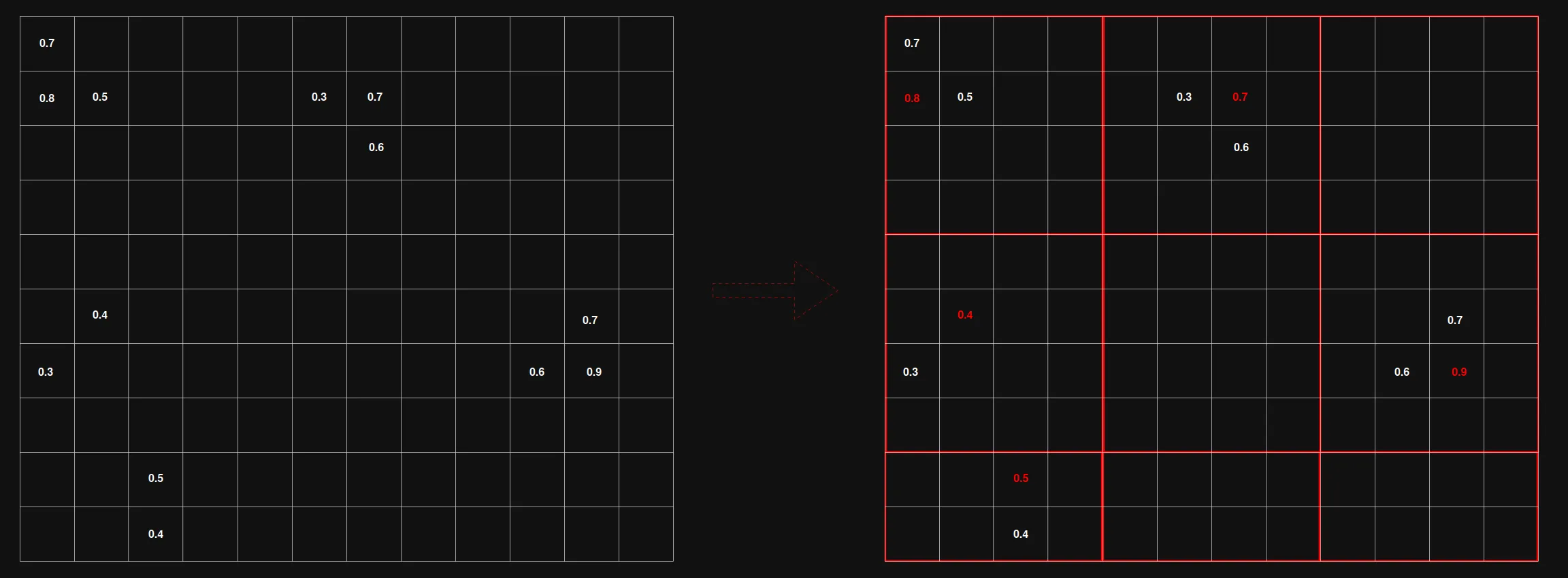
As a result, the filtered 2D proposals are then:
Position (x, y)      Score
   ( 0, 1)            0.8
   ( 6, 1)            0.7
   ( 1, 5)            0.4
   (10, 6)            0.9
   ( 2, 8)            0.5